Spectroscopy: Interaction of light and matter
Introduction to spectroscopy
Chemists study how different forms of electromagnetic radiation interact with atoms and molecules. This interaction is known as spectroscopy. Just as there are various types of electromagnetic radiation, there are various types of spectroscopy depending on the frequency of light we are using. We will begin our discussion by considering UV-Vis spectroscopy – that is, what occurs within atoms and molecules when photons in the UV and visible ranges of the spectrum (wavelengths of about \[10-700\text{ nm}\]) are absorbed or emitted.
UV-Vis spectroscopy
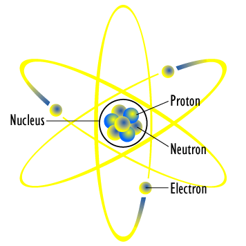
We have mentioned how atoms and molecules can absorb photons, thereby absorbing their energy. Depending on the energy of the photon absorbed or emitted, different phenomena can occur. We will start by considering the simpler case of what happens when a hydrogen atom absorbs light in the visible or UV region of the electromagnetic spectrum.
When an atom absorbs an UV photon or a photon of visible light, the energy of that photon can excite one of that atom’s electrons to a higher energy level. This movement of an electron from a lower energy level to a higher energy level, or from a higher energy back down to a lower energy level, is known as a transition. In order for a transition to occur, the energy of the photon absorbed must be greater than or equal to the difference in energy between the \[2\] energy levels. However, once the electron is in the excited, higher energy level, it is in a more unstable position than it was when it was in its relaxed, ground state. As such, the electron will quickly fall back down to the lower energy level—and it doing so, it emits a photon with an energy equal to the difference in energy levels. (To help visualize all of this, this video on YouTube provides an excellent example: https://www.youtube.com/watch?v=4jyfi28i928)
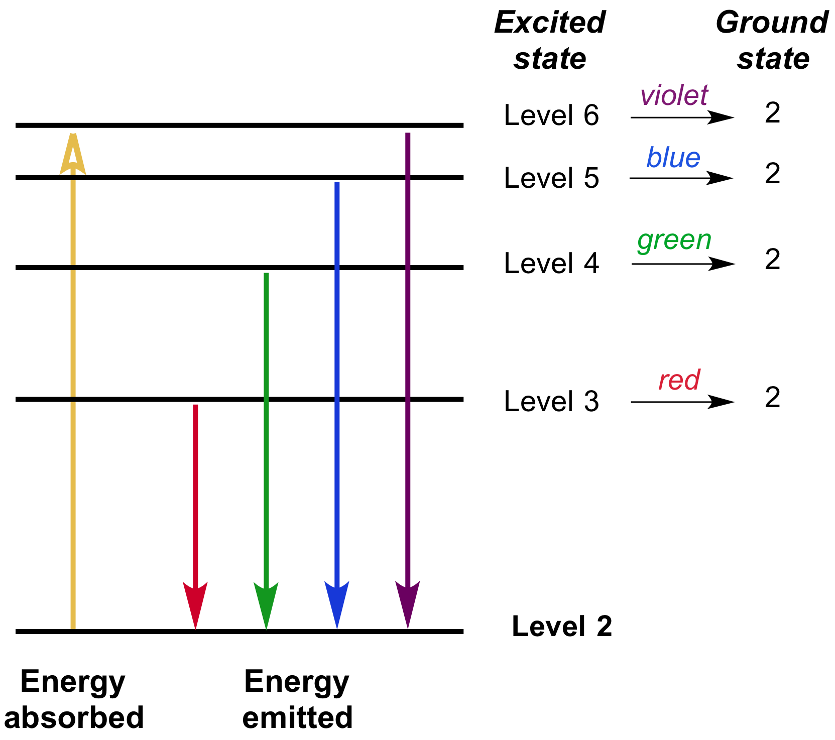
Excited electrons falling from higher energy levels down to the \[2^{\text{nd}}\] energy level in a hydrogen atom will emit photons of different frequencies, and thus different colors of light.
In the diagram above, we have a simplified picture of some of the different energy level transitions possible for our hydrogen atom. Note that the larger the transition between energy levels, the more energy is absorbed/emitted. Therefore, higher frequency photons are associated with the larger energy transitions. For example, when an electron falls from the third energy level to the second energy level, it emits a photon of red light (wavelength of about \[700\text{ nm}\]); however, when an electron falls from the sixth energy level to the second energy level (larger transition), it emits a photon of purple light (wavelength of about \[400\text{ nm}\]), which is higher in frequency (and thus greater in energy) than red light.
The energy transitions for the electrons of each element are unique, and are distinct from one another. Thus, by examining the colors of light emitted by a particular atom, we can identify that element based upon its emission spectrum. The following shows a few examples of the emission spectra for some common elements:
The atomic emission spectra for various elements. Each thin band in each spectrum corresponds to a single, unique transition between energy levels in an atom. Image from the Rochester Institute of Technology, CC BY-NC-SA 2.0.
Since each emission spectrum is unique to the element, we can think of each of these spectra as being like the “fingerprint” of each element. The thin bands indicate the particular wavelengths of light emitted when electrons in each element fall from an excited state down to a lower energy state. Scientists are able to isolate these different wavelengths by shining the light from excited atoms through a prism, which separates the different wavelengths through the process of refraction. Without a prism, however, we do not see these different wavelengths of light one at a time, but all blended together. Still, the color emitted by each element is quite distinct, which is often useful in a laboratory setting.
In the lab, we can often distinguish between elements by using a flame test. The following picture shows the characteristic green flame that appears when copper metal or copper-containing salts is burned. (Keep in mind that it is the heat energy—a type of electromagnetic radiation—that is able to excite the electrons in each atom.)
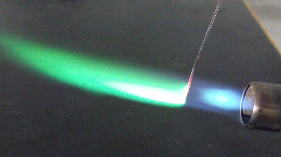
Due to the electronic transitions unique to every copper atom, copper metal burns a characteristic green color when exposed to a flame. Image from Wikipedia, CC BY-SA 3.0.
If we are testing an unknown sample in the lab to determine which elements it contains, we can always use a flame test, and draw a conclusion based on the color of flame that we see. (For more on the use of flame tests, check out this video: https://www.youtube.com/watch?v=9oYF-HxtoYg)
Infrared (IR) spectroscopy: Molecular vibrations
So far, we have been talking about electronic transitions, which occur when photons in the UV-visible range of the spectrum are absorbed by atoms. However, lower energy radiation in the infrared (IR) region of the spectrum can also produce changes within atoms and molecules. This type of radiation is usually not energetic enough to excite electrons, but it will cause the chemical bonds within molecules to vibrate in different ways. Just as the energy required to excite an electron in a particular atom is fixed, the energy required to change the vibration of a particular chemical bond is also fixed. By using special equipment in the lab, chemists can look at the IR absorption spectrum for a particular molecule, and can then use that spectrum to determine what types of chemical bonds are present in the molecule. For example, a chemist might learn from an IR spectrum that a molecule contains carbon-carbon single bonds, carbon-carbon double bonds, carbon-nitrogen single bonds, carbon-oxygen double bonds, to name but a few. Because each of these bonds is different, each will vibrate in a different way, and absorb IR radiation of different wavelengths. Thus, by looking at an IR absorption spectrum , a chemist can make some important determinations about a molecule’s chemical structure.
Spectrophotometry: The Beer-Lambert law
The last type of spectroscopy we will consider is that used to determine the concentration of solutions containing colored compounds. If you’ve ever put food coloring in water, then you already know that the more food coloring you put in, the darker and more colored your solution becomes.
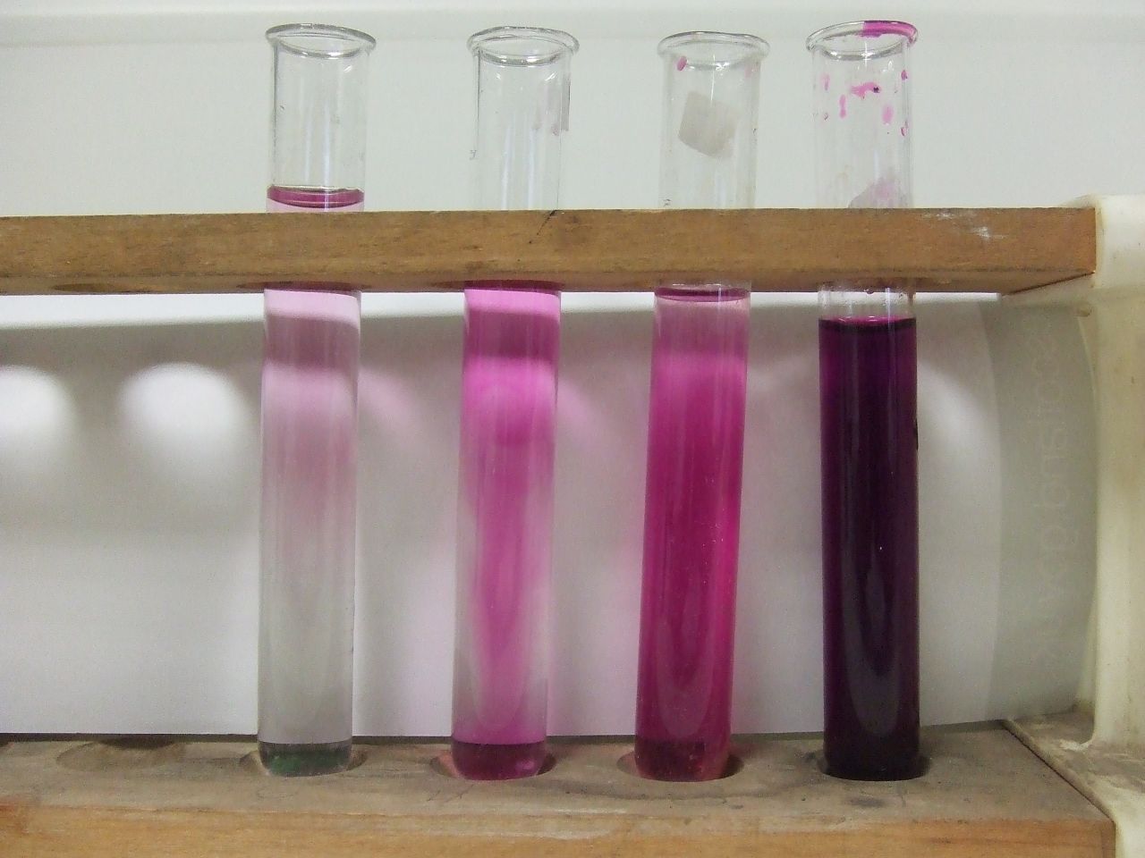
Solutions of potassium permanganate \[(\text{KMnO}_4)\] of differing concentrations. The more concentrated the solution, the darker the solution becomes, and the greater its absorbance. Image from Flickr, CC BY 2.0.
When a solution becomes darker, it means that it is absorbing more visible light. One of the most commonly used analytical techniques in chemistry is to place a solution of unknown concentration into a spectrophotometer—a device that measures the absorbance of the solution. Absorbance is measured from \[0\] to \[1\]. An absorbance of zero means that light totally passes through the solution (the solution is completely clear), and an absorbance of \[1\] means that no light passes through the solution (the solution is completely opaque). Absorbance is related to the concentration of the colored species in solution by the Beer-Lambert law, which is:
\[A=\epsilon lc\]
Where \[A\] is the absorbance (a unitless quantity), \[\epsilon\] is the molar absorptivity constant (a constant unique to each compound, given in units of \[\text{M}^{-1}\text{cm}^{-1}\]), \[l\] is the path length of the solution container (in \[\text{cm}\]), and \[c\] is the concentration of the solution in molarity \[\Big(\text{M}\], or \[\dfrac{\text{mol}}{\text{L}}\Big)\].
Example: Using the Beer-Lambert law to find the concentration of a solution
A copper (II) sulfate solution of unknown concentration is placed into a spectrophotometer. A student finds that the solution’s absorbance is \[0.462\]. The molar absorptivity of copper (II) sulfate is \[2.81\text{ M}^{-1}\text{cm}^{-1}\], and the path length of the solution container is \[1.00\text{ cm}\].
What is the concentration of the solution?
First, we can apply the Beer-Lambert Law.
\[A=\epsilon lc\]
Next, we rearrange the equation to solve for concentration, \[c\].
\[c=\dfrac{A}{\epsilon l}\]
Lastly, we can plug in our given values and solve for \[c\].
\[c=\dfrac{0.462}{(2.81\text{ M}^{-1}\cancel{\text{cm}^{-1}})\times (1.00\cancel{\text{ cm}})}=0.164\text{ M}\]
Conclusion
Photons carry discrete amounts of energy called quanta which can be transferred to atoms and molecules when photons are absorbed. Depending on the frequency of the electromagnetic radiation, chemists can probe different parts of an atom or molecule's structure using different kinds of spectroscopy. Photons in the UV or visible ranges of the EM spectrum can have sufficient energy to excite electrons. Once those electrons relax back to their ground states, photons will be emitted, and the atom or molecule will give off visible light of specific frequencies. These atomic emission spectra can be used (often informally by using a flame test) to gain insight into the electronic structure and identity of an element.
Atoms and molecules can also absorb and emit lower frequency, IR radiation. IR absorption spectra are useful to chemists because they indicate the chemical structure of a molecule, and the types of bonds it contains. Lastly, spectroscopy can also be used in the laboratory to determine the concentrations of unknown solutions, using the Beer-Lambert Law.
Photoelectric effect
Key points
Based on the wave model of light, physicists predicted that increasing light amplitude would increase the kinetic energy of emitted photoelectrons, while increasing the frequency would increase measured current.
Contrary to the predictions, experiments showed that increasing the light frequency increased the kinetic energy of the photoelectrons, and increasing the light amplitude increased the current.
Based on these findings, Einstein proposed that light behaved like a stream of particles called photons with an energy of \[\text{E}=h\nu\].
The work function, \[\Phi\], is the minimum amount of energy required to induce photoemission of electrons from a metal surface, and the value of \[\Phi\] depends on the metal.
The energy of the incident photon must be equal to the sum of the metal's work function and the photoelectron kinetic energy: \[\text{E}_\text{photon}=\text{KE}_\text{electron}+\Phi\]
Introduction: What is the photoelectric effect?
When light shines on a metal, electrons can be ejected from the surface of the metal in a phenomenon known as the photoelectric effect. This process is also often referred to as photoemission, and the electrons that are ejected from the metal are called photoelectrons. In terms of their behavior and their properties, photoelectrons are no different from other electrons. The prefix, photo-, simply tells us that the electrons have been ejected from a metal surface by incident light.
Who discovered the photoelectric effect?
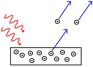
In the photoelectric effect, light waves (red wavy lines) hitting a metal surface cause electrons to be ejected from the metal. Image from Wikimedia Commons, CC BY-SA 3.0.
In this article, we will discuss how 19th century physicists attempted (but failed!) to explain the photoelectric effect using classical physics. This ultimately led to the development of the modern description of electromagnetic radiation, which has both wave-like and particle-like properties.
Predictions based on light as a wave
To explain the photoelectric effect, 19th-century physicists theorized that the oscillating electric field of the incoming light wave was heating the electrons and causing them to vibrate, eventually freeing them from the metal surface. This hypothesis was based on the assumption that light traveled purely as a wave through space. (See this article for more information about the basic properties of light.) Scientists also believed that the energy of the light wave was proportional to its brightness, which is related to the wave's amplitude. In order to test their hypotheses, they performed experiments to look at the effect of light amplitude and frequency on the rate of electron ejection, as well as the kinetic energy of the photoelectrons.
Based on the classical description of light as a wave, they made the following predictions:
The kinetic energy of emitted photoelectrons should increase with the light amplitude.
The rate of electron emission, which is proportional to the measured electric current, should increase as the light frequency is increased.
To help us understand why they made these predictions, we can compare a light wave to a water wave. Imagine some beach balls sitting on a dock that extends out into the ocean. The dock represents a metal surface, the beach balls represent electrons, and the ocean waves represent light waves.
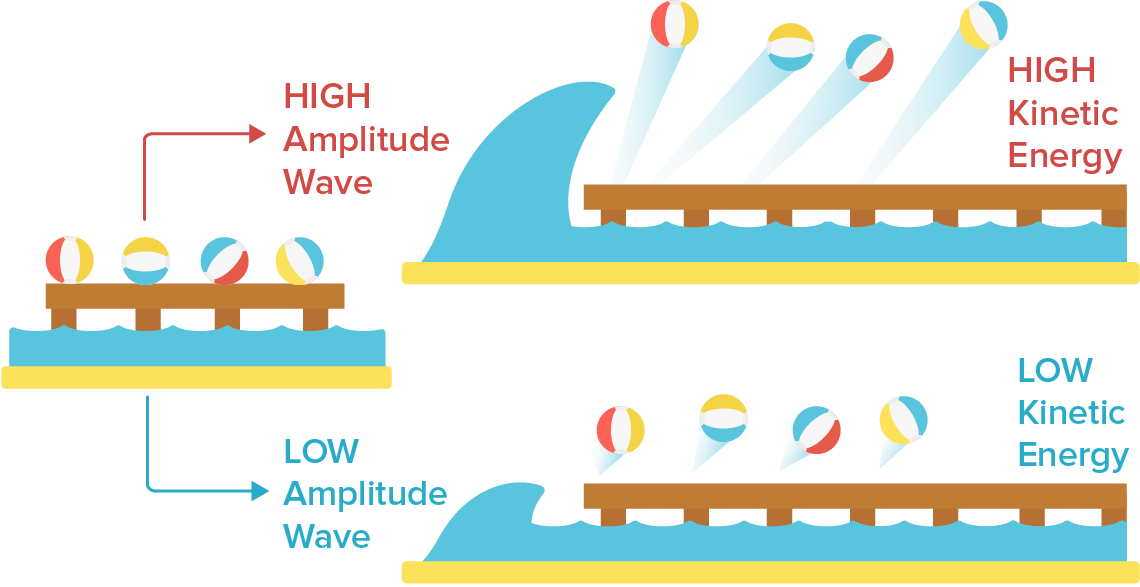
If a single large wave were to shake the dock, we would expect the energy from the big wave would send the beach balls flying off the dock with much more kinetic energy compared to a single, small wave. This is also what physicists believed would happen if the light intensity was increased. Light amplitude was expected to be proportional to the light energy, so higher amplitude light was predicted to result in photoelectrons with more kinetic energy.
Classical physicists also predicted that increasing the frequency of light waves (at a constant amplitude) would increase the rate of electrons being ejected, and thus increase the measured electric current. Using our beach ball analogy, we would expect waves hitting the dock more frequently would result in more beach balls being knocked off the dock compared to the same sized waves hitting the dock less often.
Now that we know what physicists thought would happen, let's look at what they actually observed experimentally!
When intuition fails: photons to the rescue!
When experiments were performed to look at the effect of light amplitude and frequency, the following results were observed:
The kinetic energy of photoelectrons increases with light frequency.
Electric current remains constant as light frequency increases.
Electric current increases with light amplitude.
The kinetic energy of photoelectrons remains constant as light amplitude increases.
These results were completely at odds with the predictions based on the classical description of light as a wave! In order to explain what was happening, it turned out that an entirely new model of light was needed. That model was developed by Albert Einstein, who proposed that light sometimes behaved as particles of electromagnetic energy which we now call photons. The energy of a photon could be calculated using Planck's equation:
\[\text{E}_{\text{photon}}=h\nu\]
where \[\text{E}_{\text{photon}}\] is the energy of a photon in joules (\[\text{J}\]), \[h\] is Planck's constant \[(6.626\times10^{-34}\text{ J}\cdot\text{s})\], and \[\nu\] is the frequency of the light in \[\text{Hz}\]. According to Planck's equation, the energy of a photon is proportional to the frequency of the light, \[\nu\]. The amplitude of the light is then proportional to the number of photons with a given frequency.
Concept check: As the wavelength of a photon increases, what happens to the photon's energy?
Light frequency and the threshold frequency \[\nu_0\]
We can think of the incident light as a stream of photons with an energy determined by the light frequency. When a photon hits the metal surface, the photon's energy is absorbed by an electron in the metal. The graphic below illustrates the relationship between light frequency and the kinetic energy of ejected electrons.
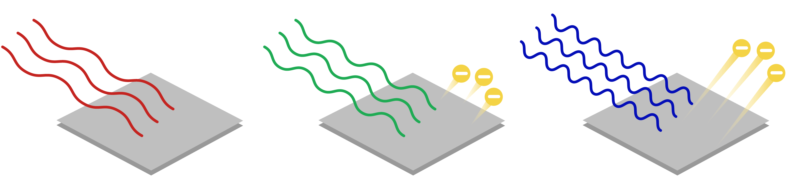
The frequency of red light (left) is less than the threshold frequency of this metal \[(\nu_\text{red}<\nu_0)\], so no electrons are ejected. The green (middle) and blue light (right) have \[\nu>\nu_0\], so both cause photoemission. The higher energy blue light ejects electrons with higher kinetic energy compared to the green light.
The scientists observed that if the incident light had a frequency less than a minimum frequency \[\nu_0\], then no electrons were ejected regardless of the light amplitude. This minimum frequency is also called the threshold frequency, and the value of \[\nu_0\] depends on the metal. For frequencies greater than \[\nu_0\], electrons would be ejected from the metal. Furthermore, the kinetic energy of the photoelectrons was proportional to the light frequency. The relationship between photoelectron kinetic energy and light frequency is shown in graph (a) below.

Because the light amplitude was kept constant as the light frequency increased, the number of photons being absorbed by the metal remained constant. Thus, the rate at which electrons were ejected from the metal (or the electric current) remained constant as well. The relationship between electron current and light frequency is illustrated in graph (b) above.
Isn't there more math somewhere?
We can analyze the frequency relationship using the law of conservation of energy. The total energy of the incoming photon, \[\text{E}_\text{photon}\], must be equal to the kinetic energy of the ejected electron, \[\text{KE}_{\text{electron}}\], plus the energy required to eject the electron from the metal. The energy required to free the electron from a particular metal is also called the metal's work function, which is represented by the symbol \[\Phi\] (in units of \[\text J\]):
\[\text{E}_\text{photon}=\text{KE}_\text{electron}+\Phi\]
Like the threshold frequency \[\nu_0\], the value of \[\Phi\] also changes depending on the metal. We can now write the energy of the photon in terms of the light frequency using Planck's equation:
\[\text{E}_\text{photon}=h\nu=\text{KE}_\text{electron}+\Phi\]
Rearranging this equation in terms of the electron's kinetic energy, we get:
\[\text{KE}_\text{electron}=h\nu-\Phi\]
We can see that kinetic energy of the photoelectron increases linearly with \[\nu\] as long as the photon energy is greater than the work function \[\Phi\], which is exactly the relationship shown in graph (a) above. We can also use this equation to find the photoelectron velocity \[\text v\], which is related to \[\text{KE}_\text{electron}\] as follows:
\[\text{KE}_\text{electron}=h\nu-\Phi=\dfrac{1}{2}m_e\text v^2\]
where \[m_e\] is the rest mass of an electron, \[9.1094 \times 10^{-31} \,\text{kg}\].
Exploring the wave amplitude trends
In terms of photons, higher amplitude light means more photons hitting the metal surface. This results in more electrons ejected over a given time period. As long as the light frequency is greater than \[\nu_0\], increasing the light amplitude will cause the electron current to increase proportionally as shown in graph (a) below.

Since increasing the light amplitude has no effect on the energy of the incoming photon, the photoelectron kinetic energy remains constant as the light amplitude is increased (see graph (b) above).
If we try to explain this result using our dock-and-beach-balls analogy, the relationship in graph (b) indicates that no matter the height of the wave hitting the dock\[-\]whether it's a tiny swell, or a huge tsunami\[-\]the individual beach balls would be launched off the dock with the exact same speed! Thus, our intuition and analogy don't do a very good job of explaining these particular experiments.
Example \[1\]: The photoelectric effect for copper
The work function of copper metal is \[\Phi=7.53\times10^{-19}\text{ J}\]. If we shine light with a frequency of \[3.0\times 10^{16}\text{ Hz}\] on copper metal, will the photoelectric effect be observed?
In order to eject electrons, we need the energy of the photons to be greater than the work function of copper. We can use Planck's equation to calculate the energy of the photon, \[\text{E}_{\text{photon}}\]:
\[\begin{aligned} \text{E}_\text{photon} &= h\nu \\
&= (6.626\times10^{-34}\text{ J}\cdot\text{s})(3.0\times10^{16}\text{ Hz}) ~~~~\text{plug in values for $h$ and $\nu$}\\
&= 2.0\times10^{-17}\text{ J} \end{aligned}\]
If we compare our calculated photon energy, \[\text{E}_\text{photon}\], to copper's work function, we see that the photon energy is greater than \[\Phi\]:
\[~2.0\times10^{-17}\text{ J}~>~7.53\times10^{-19}\text{ J}\]
\[~~~~~~~~\text{E}_\text{photon}~~~~~~~~~~~~~~~~~~~\Phi\]
Thus, we would expect to see photoelectrons ejected from the copper. Next, we will calculate the kinetic energy of the photoelectrons.
Example \[2\]: Calculating the kinetic energy of a photoelectron
What is the kinetic energy of the photoelectrons ejected from the copper by the light with a frequency of \[3.0\times 10^{16}\text{ Hz}\]?
We can calculate the kinetic energy of the photoelectron using the equation that relates \[\text{KE}_\text{electron}\] to the energy of the photon, \[\text{E}_\text{photon}\], and the work function, \[\Phi\]:
\[\text{E}_\text{photon}=\text{KE}_\text{electron}+\Phi\]
Since we want to know \[\text{KE}_\text{electron}\], we can start by rearranging the equation so that we will be solving for the kinetic energy of the electron:
\[\text{KE}_\text{electron}=\text{E}_\text{photon}-\Phi\]
Now we can insert our known values for \[\text{E}_\text{photon}\] and \[\Phi\] from Example 1:
\[\text{KE}_\text{electron}=(2.0\times10^{-17}\text{ J})-(7.53\times10^{-19}\text{ J})=1.9\times10^{-17}\text{ J}\]
Therefore, each photoelectron has a kinetic energy of \[1.9\times10^{-17}\text{ J}\].
Summary
Based on the wave model of light, physicists predicted that increasing light amplitude would increase the kinetic energy of emitted photoelectrons, while increasing the frequency would increase measured current.
Experiments showed that increasing the light frequency increased the kinetic energy of the photoelectrons, and increasing the light amplitude increased the current.
Based on these findings, Einstein proposed that light behaved like a stream of photons with an energy of \[\text{E}=h\nu\].
The work function, \[\Phi\], is the minimum amount of energy required to induce photoemission of electrons from a specific metal surface.
The energy of the incident photon must be equal to the sum of the work function and the kinetic energy of a photoelectron: \[\text{E}_\text{photon}=\text{KE}_\text{electron}+\Phi\
Try it!
When we shine light with a frequency of \[6.20 \times 10^{14}\,\text{Hz}\] on a mystery metal, we observe the ejected electrons have a kinetic energy of \[3.28\times 10^{-20}\,\text J\]. Some possible candidates for the mystery metal are shown in the table below:
| Metal | Work function \[\Phi\] (Joules, \[\text J\]) |
|---|---|
| Calcium, \[\text{Ca}\] | \[4.60\times 10^{-19}\] |
| Tin, \[\text{Sn}\] | \[7.08\times 10^{-19}\] |
| Sodium, \[\text{Na}\] | \[3.78\times 10^{-19}\] |
| Hafnium, \[\text{Hf}\] | \[6.25\times 10^{-19}\] |
| Samarium, \[\text{Sm}\] | \[4.33\times 10^{-19}\] |
Photoelectric effect
Key points
Bohr's model of hydrogen is based on the nonclassical assumption that electrons travel in specific shells, or orbits, around the nucleus.
Bohr's model calculated the following energies for an electron in the shell, \[n\]:
\[E(n)=-\dfrac{1}{n^2} \cdot 13.6\,\text{eV}\]
- Bohr explained the hydrogen spectrum in terms of electrons absorbing and emitting photons to change energy levels, where the photon energy is
\[h\nu =\Delta E = \left(\dfrac{1}{{n_{low}}^2}-\dfrac{1}{{n_{high}}^2}\right) \cdot 13.6\,\text{eV} \]
- Bohr's model does not work for systems with more than one electron.
The planetary model of the atom
At the beginning of the 20th century, a new field of study known as quantum mechanics emerged. One of the founders of this field was Danish physicist Niels Bohr, who was interested in explaining the discrete line spectrum observed when light was emitted by different elements. Bohr was also interested in the structure of the atom, which was a topic of much debate at the time. Numerous models of the atom had been postulated based on experimental results including the discovery of the electron by J. J. Thomson and the discovery of the nucleus by Ernest Rutherford. Bohr supported the planetary model, in which electrons revolved around a positively charged nucleus like the rings around Saturn—or alternatively, the planets around the sun.

Many scientists, including Rutherford and Bohr, thought electrons might orbit the nucleus like the rings around Saturn. Image credit: Image of Saturn by NASA
However, scientists still had many unanswered questions:
Where are the electrons, and what are they doing?
If the electrons are orbiting the nucleus, why don’t they fall into the nucleus as predicted by classical physics?
Why does classical physics predict that?
How is the internal structure of the atom related to the discrete emission lines produced by excited elements?
Bohr addressed these questions using a seemingly simple assumption: what if some aspects of atomic structure, such as electron orbits and energies, could only take on certain values?
Quantization and photons
By the early 1900s, scientists were aware that some phenomena occurred in a discrete, as opposed to continuous, manner. Physicists Max Planck and Albert Einstein had recently theorized that electromagnetic radiation not only behaves like a wave, but also sometimes like particles called photons. Planck studied the electromagnetic radiation emitted by heated objects, and he proposed that the emitted electromagnetic radiation was "quantized" since the energy of light could only have values given by the following equation: \[E_{\text{photon}}=nh\nu\], where \[n\] is a positive integer, \[h\] is Planck’s constant—\[6.626 \times10^{-34}\,\text{J}\cdot \text s\]—and \[\nu\] is the frequency of the light, which has units of \[\dfrac{1}{\text s}\].
As a consequence, the emitted electromagnetic radiation must have energies that are multiples of \[h\nu\]. Einstein used Planck's results to explain why a minimum frequency of light was required to eject electrons from a metal surface in the photoelectric effect.
Where can I learn more about the photoelectric effect?
When something is quantized, it means that only specific values are allowed, such as when playing a piano. Since each key of a piano is tuned to a specific note, only a certain set of notes—which correspond to frequencies of sound waves—can be produced. As long as your piano is properly tuned, you can play an F or F sharp, but you can't play the note that is halfway between an F and F sharp.
Atomic line spectra
Atomic line spectra are another example of quantization. When an element or ion is heated by a flame or excited by electric current, the excited atoms emit light of a characteristic color. The emitted light can be refracted by a prism, producing spectra with a distinctive striped appearance due to the emission of certain wavelengths of light.
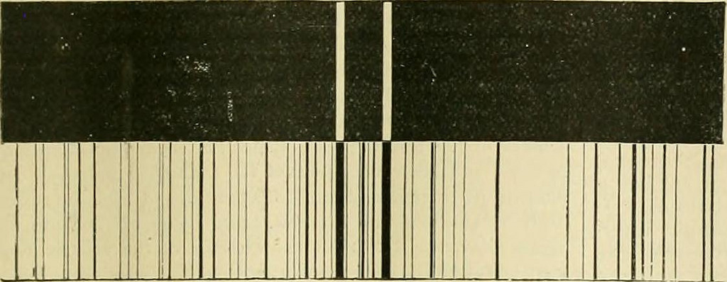
Emission spectra of sodium, top, compared to the emission spectrum of the sun, bottom. The dark lines in the emission spectrum of the sun, which are also called Fraunhofer lines, are from absorption of specific wavelengths of light by elements in the sun's atmosphere. The side-by-side comparison shows that the pair of dark lines near the middle of the sun's emission spectrum are probably due to sodium in the sun's atmosphere. Image credit: From the Biodiversity Heritage Library
For the relatively simple case of the hydrogen atom, the wavelengths of some emission lines could even be fitted to mathematical equations. The equations did not explain why the hydrogen atom emitted those particular wavelengths of light, however. Prior to Bohr's model of the hydrogen atom, scientists were unclear of the reason behind the quantization of atomic emission spectra.
Bohr's model of the hydrogen atom: quantization of electronic structure
Bohr’s model of the hydrogen atom started from the planetary model, but he added one assumption regarding the electrons. What if the electronic structure of the atom was quantized? Bohr suggested that perhaps the electrons could only orbit the nucleus in specific orbits or shells with a fixed radius. Only shells with a radius given by the equation below would be allowed, and the electron could not exist in between these shells. Mathematically, we could write the allowed values of the atomic radius as \[r(n)=n^2\cdot r(1)\], where \[n\] is a positive integer, and \[r(1)\] is the Bohr radius, the smallest allowed radius for hydrogen.
He found that \[r(1)\] has the value
\[\text{Bohr radius}=r(1)=0.529 \times 10^{-10} \,\text{m}\]
An atom of lithium shown using the planetary model. The electrons are in circular orbits around the nucleus. Image credit: planetary atomic model from Wikimedia Commons, CC-BY-SA 3.0
By keeping the electrons in circular, quantized orbits around the positively-charged nucleus, Bohr was able to calculate the energy of an electron in the \[n\]th energy level of hydrogen: \[E(n)=-\dfrac{1}{n^2} \cdot 13.6\,\text{eV}\], where the lowest possible energy or ground state energy of a hydrogen electron—\[E(1)\]—is \[-13.6\,\text{eV}\].
Note that the energy is always going to be a negative number, and the ground state, \[n=1\], has the most negative value. This is because the energy of an electron in orbit is relative to the energy of an electron that has been completely separated from its nucleus, \[n=\infty\], which is defined to have an energy of \[0\,\text{eV}\]. Since an electron in orbit around the nucleus is more stable than an electron that is infinitely far away from its nucleus, the energy of an electron in orbit is always negative.
Absorption and emission
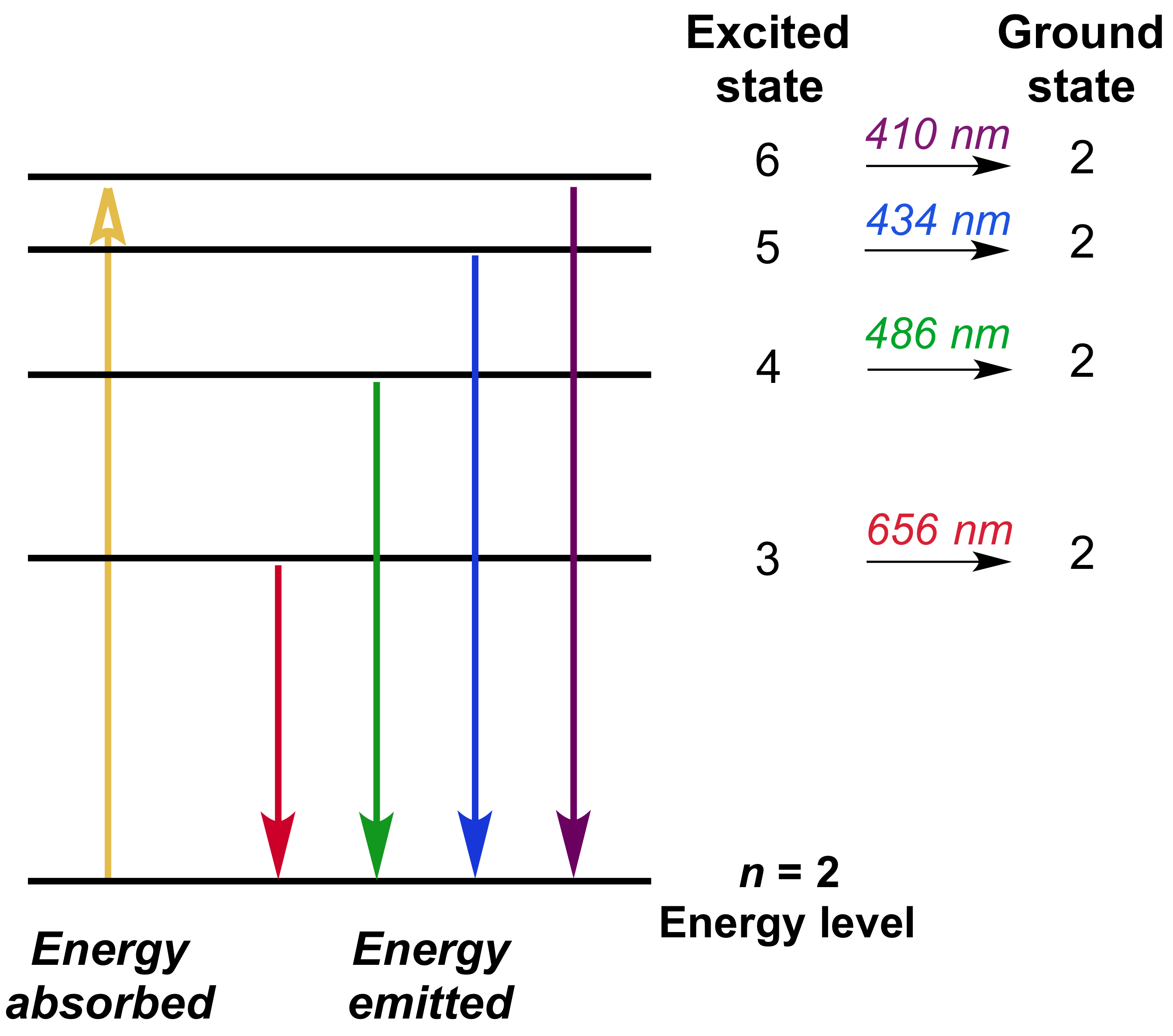
The Balmer series—the spectral lines in the visible region of hydrogen's emission spectrum—corresponds to electrons relaxing from n=3-6 energy levels to the n=2 energy level.
Bohr could now precisely describe the processes of absorption and emission in terms of electronic structure. According to Bohr's model, an electron would absorb energy in the form of photons to get excited to a higher energy level as long as the photon's energy was equal to the energy difference between the initial and final energy levels. After jumping to the higher energy level—also called the excited state—the excited electron would be in a less stable position, so it would quickly emit a photon to relax back to a lower, more stable energy level.
The energy levels and transitions between them can be illustrated using an energy level diagram, such as the example above showing electrons relaxing back to the \[n=2\] level of hydrogen. The energy of the emitted photon is equal to the difference in energy between the two energy levels for a particular transition. The energy difference between energy levels \[n_{high}\] and \[n_{low}\] can be calculated using the equation for \[E(n)\] from the previous section:
\[\begin{aligned} \Delta E &= E(n_{high})-E(n_{low}) \\
\\
&=\left( -\dfrac{1}{{n_{high}}^2} \cdot 13.6\,\text{eV} \right)-\left(-\dfrac{1}{{n_{low}}^2} \cdot 13.6\,\text{eV}\right) \\
\\
&= \left(\dfrac{1}{{n_{low}}^2}-\dfrac{1}{{n_{high}}^2}\right) \cdot 13.6\,\text{eV} \end{aligned}\]
Since we also know the relationship between the energy of a photon and its frequency from Planck's equation, we can solve for the frequency of the emitted photon:
\[\begin{aligned} h\nu &=\Delta E = \left(\dfrac{1}{{n_{low}}^2}-\dfrac{1}{{n_{high}}^2}\right) \cdot 13.6\,\text{eV} ~~~~~~~~~~~~\text{Set photon energy equal to energy difference}\\
\\
\nu &= \left(\dfrac{1}{{n_{low}}^2}-\dfrac{1}{{n_{high}}^2}\right) \cdot \dfrac{13.6\,\text{eV}}{h}~~~~~~~~~~~~~~~~~~~~~~\text{Solve for frequency}\end{aligned}\]
We can also find the equation for the wavelength of the emitted electromagnetic radiation using the relationship between the speed of light \[\text c\], frequency \[\nu\], and wavelength \[\lambda\]:
\[\begin{aligned}\text c &=\lambda \nu ~~~~~~~~~~~~~~~~~~~~~~~~~~~~~~~~~~~~~~~~~~~~~~~~~~~~~~~~~~~~~~~~~~\text{Rearrange to solve for }\nu . \\\\
\dfrac{\text c}{\lambda}&=\nu=\left(\dfrac{1}{{n_{low}}^2}-\dfrac{1}{{n_{high}}^2}\right) \cdot \dfrac{13.6\,\text{eV}}{h}~~~~~~~~~~~~~~\text{Divide both sides by c to solve for }\dfrac{1}{\lambda}.\\\\
\\\\
\dfrac{1}{\lambda} &=\left(\dfrac{1}{{n_{low}}^2}-\dfrac{1}{{n_{high}}^2}\right) \cdot \dfrac{13.6\,\text{eV}}{h\text c} \end{aligned}\]
What about the Rydberg constant?
Thus, we can see that the frequency—and wavelength—of the emitted photon depends on the energies of the initial and final shells of an electron in hydrogen.
What have we learned since Bohr proposed his model of hydrogen?
The Bohr model worked beautifully for explaining the hydrogen atom and other single electron systems such as \[\text{He}^+\]. Unfortunately, it did not do as well when applied to the spectra of more complex atoms. Furthermore, the Bohr model had no way of explaining why some lines are more intense than others or why some spectral lines split into multiple lines in the presence of a magnetic field—the Zeeman effect.
In the following decades, work by scientists such as Erwin Schrödinger showed that electrons can be thought of as behaving like waves and behaving as particles. This means that it is not possible to know both a given electron’s position in space and its velocity at the same time, a concept that is more precisely stated in Heisenberg's uncertainty principle. The uncertainty principle contradicts Bohr’s idea of electrons existing in specific orbits with a known velocity and radius. Instead, we can only calculate probabilities of finding electrons in a particular region of space around the nucleus.
The modern quantum mechanical model may sound like a huge leap from the Bohr model, but the key idea is the same: classical physics is not sufficient to explain all phenomena on an atomic level. Bohr was the first to recognize this by incorporating the idea of quantization into the electronic structure of the hydrogen atom, and he was able to thereby explain the emission spectra of hydrogen as well as other one-electron systems.